Economic schools

Classical

1. Key Players: Adam Smith, John B. Say, David Ricardo, Alfred Marshall
2. Supply creates its own demand (whatever output is produced will be demanded
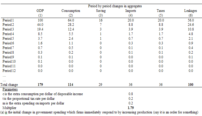
3. Savings are leakages
4. Investments are injections
5. Aggregate Supply determines output
6. "Invisible Hand" - Where market functions by itself, no government intervention (laissez-faire)
7. Savings increase with the interest rate
8. Aggregate Supply = Aggregate Demand at full employment equilibrium
9. In the long-run, the economy will balance at full employment
10. The economy is always close to or at full employment
11. "Trickle-Down Effect" - Help the rich first, and the poor will benefit later. Much later.
12. Prices and wages are flexible downward

Keynesian

• Savers do not equal investors
• Key Player: John Maynard Keynes 
• Competition is flawed, Aggregate Demand is key, not Aggregate Supply
• Aggregate Demand determines output, demand creates its own supply
• Savers and investors save and invest for different reasons
• Savings are inverse to interest rates
• Leaks cause constant recessions
• Savings cause recessions
• Ratchet effects and stick wages block Say's Law
• Prices and wages are inflexible downward
• There is no mechanism capable of guaranteeing full employment
• In the long run, we're dead
• Economy is not close to or at full employment
• Some government intervention is needed
• Stabilizers
• Use expansionary/contractionary policy
• Fiscal policy

Monetary

1. Key Players: Alan Greenspan, Ben Bernanke
2. Fine-tuning is needed
3. Congress can't time the policy options
4. Voters won't allow contractionary options
5. Uses tight money and easy money
6. Change required reserves if needed
7. Buy and sell bonds on the open market
8. Change interest rates for discount rate and federal fund rate

Fiscal policy

Discretionary- increasing or  decreasing government spending and taxes in order to return the economy to full employment. Involves policy makers doing fiscal policy in response to an economic problem.

-Automatic- unemployment. Compensation and marginal tax rates are examples of automatic policies that help mitigate the effects of recession and inflation. Automatic fiscal policy takes place without policy makers having to respond to current economic problems.

-Contractionary fiscal policy- policy designed to decrease aggregate demand

• strategy for controlling inflation

- Expansionary fiscal policy- policy designed to increased aggregate demand

• Strategy for increasing GDP, combAtting a recession &reducing unemployment

• increase government spending (G)

• decrease taxes (T)

-Contractionary fiscal policy

Anything that increases the government budget deficit during a recession and increases its budget surplus during inflation without requiring explicit action by policymakers.

- Transfer payment: welfare checks, food stamps, unemployment checks, corporate dividends, social security, veteran's benefits

2. Progressive income taxes

automatic stabilizers take 33-50% out.

Stabilizers are like a thermostat maintaining temperature. They are shock absorbers.

- Progressive tax system

• average tax rate ( tax revenue/ GDP) rises with GSP

-Proportional tax system

• average tax rate remains constant as GDP changes

- Regressive tax system

• Average tax rate falls with GDP

Disposable income and Multiplier's

Disposable Income (DI)

1. Income after taxes or net income
2. DI = Gross Income - Taxes

2 Choices

1. With disposable income, households can either
1. Consume (spend money on goods and services)
2. Save (not spend money on goods and services)

Consumption

• Household spending
• The ability to consume is constrained by:
• The amount of disposable income
• The propensity to save
• Do households consume if DI = 0?
• Autonomous consumption
• Dissaving
• APC = C/DI = % DI that is spent

Saving

• Household NOT spending
• The ability to save is constrained by:
• The amount of DI
• The propensity to consume
• Do households save if DI = 0? No.
• APS = S/DI = % DI that is not spent

APC & APS

• APC + APS = 1
• 1 - APC = APS
• 1 - APS = APC
• APC > 1 : Dissaving
• - APS . Dissaving

MPC and MPS

• Marginal Propensity to Consume
• △C/△DI
• % of every extra dollar earned that is spent
• Marginal Propensity to Save
• △S/△DI
• % of every extra dollar earned that is saved
• MPC + MPS = 1
• 1 - MPC = MPS
• 1 - MPS = MPC

The Spending Multiplier Effect

• An initial change in spending (C, G, Ig, Xn) causes larger change in aggregate spending (or AD)
• Multiplier = △in AD/△in spending
• Multiplier = △in AD/△C, G, Ig, Xn

• Why does this happen?
• Expenditures and income flow continuously which then sets off a spending increase in the economy

• Can be calculated from MPC or MPS
• Multiplier = 1/1-MPC or 1/MPS
• Multipliers are + when there is an increase in spending and - when there is a decrease

Tax Multiplier

• When government taxes, multiplier works in reverse b/c money is leaving circular flow
• Tax Multiplier Formula (it's negative) = -MPC/1-MPC or -MPC/MPS
• If there is a tax CUT, multiplier is + because there is now more money in the circular flow

Full employment

Full Employment - FE Equilibrium exists where AD intersects SRAS and LRAS at the same point

Recessionary Gap - Exists when equilibrium occurs below full employment output, AD increases

Inflationary Gap - Exists when equilibrium occurs beyond FE output, AD increases
u - Stands for unemployment
pi - Inflation

LRAS - Vertical line at an output level that represents the quantity of goods and services a nation can produce over sustained period using all of its productive resources as efficiently as possible with all of the current tech available to it 

1. Stable at full employment 
2. LRAS curve represents a point on an economy's PPC 
3. Synonymous with PPF curving outward (change in resource, tech, economic growth)
4. Doesn't change as price level changes

Interest Rates and Investment Demands

Interest rates & Investment demand

-What is Investment

• money spent or expenditures on:

-New plants ( factories)

-capital equipment (machinery)

-technology (hardware and software)

- new homes

- inventories( goods sold by producers)

-EXPECTED RATES OF RETURNS

• how does business make investment decisions?

~cost and benefit analysis

• how does business determine the benefits?

~ expected rate of return

• how does business count the cost?

~ interest costs

•how does business determine the amount of investment they undertake

~ compare expected rate of return to interest cost

~ if expected return > interest cost, then invest

~ if expected return < interest cost, then do not invest

- real(r%) vs nominal (i%)

• whats the difference

~ nominal is the observable rate of interest. Real subtracts out of inflation (pi%) is only known ex post fact

• how do you compute the real interest rate(r%)?

r%= i% - pi%

• what then , determines the cost of an investment decision?

-the real interest rate (r%)

- INVESTMENT DEMAND CURVE (ID)

• what is the shape of the investment demand curve

~ downward sloping

•why?

~ when interest rates are high, fewer investments are profitable; when interest are low, more investments are profitable

- SHIFTS IN INVESTMENT DEMAND(ID)

-cost of production

• lower cost shift ID->

• higher cost shift ID<-

- business taxes

• lower business taxes shift ID->

• higher business taxes shift ID<-

- Technological change

• new technology shift ID->

• lack of technological change shifts ID <-

-Stocks of capital

• if an economy is low on capita then ID->

• if an economy has much capital then ID<-

-Expectations

•positive expectations shift ID->

•negative expectations shift ID<-

-LONG RUN AS- it is a vertical line on output level that represents the quantity of goods and services a nation can produces over a sustain period using all of its productive resources as efficiently as possible with all of the current technology available to it.

-LRAS- is stable at full employment

-LRAS CURVE- represents a point on a economy production possibility curve

-changes in resources, economic growth, 

-does not change as the price level changes

Aggregate supply

Aggregate supply

• the level of real GDP (GDP R) that firms will produce at each price level(PL)

Long-run: period of time where input prices are completely flexible and adjust to changes in the price-level.

• in the long run the level of real GDP supplied is independent of the price level

Short-run: period of time where input prices are sticky and do not adjust to changes in the price level

• in the short-run, the level of REAL GDP supplied is directly related to the price level

-Long-run aggregate supply (LRAS)

• the long-run aggregate supply or LRAS marks the level of full employment in the economy(analogous to PPC)

• because input prices are completely flexible in the long-run, changes in price-level do not change firms' real profits and therefore do not change firms' level of output. This means that the LRAS is vertical at the economy's level of full employment.

- Short run aggregate supply(SRAS) 

• because input prices are sticky in the short run, the SRAS is upward sloping.

- Changes in SRAS 

• an increase in SRAS IS SEEN AS A SHIFT TO THE RIGHT. SRAS->

• a decrease in SRAS is seen as a shift to the left. SRAS<-

• The key to understanding shifts in SRAS  is per unit cost of production

•Per unit production cost= total input cost/ total output

-Determinants of SRAS( all of the following affect unit of production)

•input prices

•productivity

• legal-institutional environment

-Input prices

• domestic resources prices

~ wages (75% of all business costs)

~ cost of capital

~ raw materials(commodity prices)

• Foreign resources prices

~ strong$ = lower foreign resource prices

~ weak$= higher foreign resources prices

•market power

~monopolies and cartels that control resources control the price of those resources

• increase in resource prices= SRAS <-

•decrease in resource prices= SRAS->

-Productivity

• productivity= total output/ total inputs

• more productivity = lower unit production cost=SRAS->

•lower productivity = higher unit production cost=SRAS<-

- Legal-Institutional Environment

• taxes and Subsidies

~ taxes ($ to gov't) on business increase per unit production cost= SRAS<-

~ subsidies($ from gov't) to business reduce per unit production cost= SRAS->

• Government regulation

~ government regulation creates a cost of compliance=SRAS<-

~ Deregulation reduces compliance costs= SRAS->

Aggregate Demand

1. Aggregate Demand - Shows amount of real GDP that the private, public and foreign a sector collectively desire to purchase at each possible price level
2. The relationship between price level and level of real GDP is inverse

The Reason AD is Downward Sloping

1. Real-Balances Effect
1. When price level is high, households and businesses can not afford to purchase as much output
2. When price level is low, households and businesses can afford to purchase more output 
2. Interest-Rate Effect
1. A higher price level increases interest rate, which tends to discourage investment
2. A lower price level decreases interest rate, which tends to encourage investment 
3. Foreign Purchases Effect
1. Higher price level increases demand for relatively cheaper imports
2. Lower price level increases foreign demand for cheaper US exports 
4. Shifts in Aggregate Demand
5. There are two parts to a shift in AD:
1. Change in C, Ig, G and Xn
2. Multiplier effect that produces greater change than original change in the 4 components
6. Increases in AD go right
7. Decreases go left
8. Determinants of AD

Consumption

1. Household spending is affected by:
1. Consumer Wealth
1. More wealth, more spending (AD increases)
2. Less wealth, less spending (AD decreases)

1. Consumer Expectations
1. Positive expectations - more spending 
2. Negative expectations - less spending 

1. Household Indebtedness 
1. Less debt, more spending 
2. More debt, less spending 

1. Taxes
1. Less taxes, more spending
2. More taxes, less spending 

1. Gross Private Investment

1. Investment spending is sensitive to:
1. The Real Interest Rate
1. Lower interest rate, more investment (AD increases)
2. Higher interest rate, less investment (AD decreases)

1. Expected Returns
1. Higher expected returns, more investment
2. Lower expected returns, less investment 

1. Expected returns are influenced by: 

1. Expectations of future profitability
2. Technology
3. Degree of excess capacity (Existing Stock of Capital)
4. Business Taxes

Government Spending

1. More government spending, AD increases
2. Less government spending, AD decreases

Net Exports

1. Net Exports are sensitive to:
1. Exchange Rates (International value of $)
1. Strong $ = More imports and fewer exports (AD decreases)
2. Weak $ = Fewer imports and more exports (AD increases) 

1. Relative Income
1. Strong foreign economies = more exports, AD increases
2. Weak foreign economies = less exports, AD decreases